Preprocessing Data for Spatial Analysis with PostGIS and PL/R
This is the second in a series of posts intended to introduce PostgreSQL users to PL/R, a loadable procedural language that enables a user to write user-defined SQL functions in the R programming language. This post builds on the example introduced in the initial post by demonstrating the steps associated with preprocessing the Normalized Difference Vegetation Index (NDVI) satellite raster data in preparation for spatial analytics.
The first post in this series provided users with an introduction, and discussed acquisition of administrative area boundary polygons (USA states and counties) and geocoding using PostGIS, R and PL/R. This post will walk through preprocessing of NDVI satellite raster data in preparation for spatial analytics. The forthcoming final post of this series will provide sample use of R Functions against the NDVI dataset.
As introduced in the initial post, the combination of PostGIS and R provides users with the ability to leverage the power and efficiency of the worlds most advanced open source database to perform powerful spatial analytics using the rich analytic functionality of R.
Example Overview and Setup
This series of posts uses NDVI data from the moderate-resolution imaging spectroradiometer (MODIS) made available by the United States Geologic Survey (USGS). This data is used to demonstrate analytic operations including:
- Determining Average NDVI for a Particular Location Over Time
- Visualize Average NDVI for a Particular Location Over Time with ggplot
- Visualize Average NDVI for a Particular Location by Month
- Visualize Same Month Average NDVI for a Particular Location by Year
For information regarding the background for this analysis and the example set up, please take a moment to review the initial post in this series.
Plotting Points of Interest
The initial post in this series demonstrated the process of acquiring the geometric shapes representing administrative boundaries, specifically USA states and counties, and storing those as a spatial multipolygon layer. Further, we saw how to geocode airport address data, providing a “Points of Interest” spatial points layer. With the geocoding complete, it is possible to use an R function to plot both the San Diego county administrative boundaries and the Points of Interest layer we just created. The R function used in this example is suitable for use during interactive data exploration from an R client. It is worth noting that while this example uses a pure R function, this R function can be trivially converted to a PL/R function by replacing the R function decoration syntax (function name, arguments, end of function) with those of PostgreSQL.
The R function that implements the steps described above is as follows:
# Note: this is pure R code
plot_poi <- function(plotfile, aoilayer, aoiname1, aoiname2, poilayer) {
  library(sp); library(raster);
  library(rgeos);
  library(rgdal)
  library(RPostgreSQL)
  Sys.setenv("DISPLAY"=":0.0")

  # required in R, noop in PL/R
  conn <- dbConnect(dbDriver("PostgreSQL"), user="postgres", dbname="gis", host="localhost")

  # plot to file if destination filename given
  if (plotfile != "") png(plotfile, width = 1024, height = 768)

  # retrieve boundaries for requested admin area
  p4str <- "+proj=longlat +datum=WGS84 +no_defs +ellps=WGS84 +towgs84=0,0,0"
  sql.str <- sprintf("SELECT st_astext(wkb_geometry) AS geom
                      FROM %s WHERE name_1 = '%s' and name_2 = '%s'",
                      aoilayer, aoiname1, aoiname2)
  sdc <- readWKT(dbGetQuery(conn, sql.str), p4s=p4str)

  # add county boundaries to plot
  plot(sdc)

  # retrieve points of interest
  dsn <- "PG:user='postgres' dbname='gis' host='localhost'"
  poi <- readOGR(dsn=dsn, poilayer, stringsAsFactors = FALSE)

  # add poi to plot
  plot(poi, col = "red", pch = 16, add = TRUE)
  if (plotfile != "") dev.off()
}

plot_poi("/tmp/airports1.png", "airports", "counties", "California", "San Diego")
The plot_poi() code above illustrates a different approach compared to the
first post in this series for the creation of the png image. Instead of
capturing the png image to an in-memory buffer and returning it as the function
result, the example above either (i) writes the image directly to file when a
filename is provided as one of the function's arguments, or (ii) interactively
“pops up” the image on the screen to the user running the function. Note also
that the argument add = TRUE is included in the second call to the plot()
function in order to add an additional spatial layer to the resulting image
rather than simply replacing the first layer with the second. The resulting
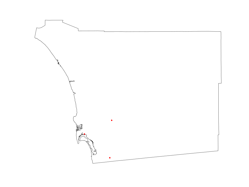
image following the plotting of the airport address data is provided in Figure 1
below.
Figure 1: Visual Results of Plotting Airport Data Points of Interest
Ingest Normalized Difference Vegetation Index (NDVI) Data
At this point, we are ready to obtain, process, and ingest the NDVI data from the MODIS satellite. In order to get started, first a login must be created at the USGS website. After logging into the myUSGS, it is possible to select and download the NDVI data necessary to complete this example using the following search criteria:
- Predefined Area : Add Shape ⇒ State ⇒ CA ⇒ County ⇒ Alameda County
- Date Range: From 2000-01-01 ⇒ To 2016-12-31
- Result Options: Number of records to return ⇒ 2000
- Data Sets: Vegetation Monitoring ⇒ eMODIS NDVI ( MOD13A1)
- Additional Criteria: Platform ⇒ TERRA
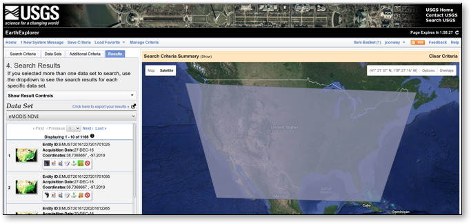
The USGS Search Criteria User Interface is shown in Figure 2 below.
Note that in this case we use “Alameda County” instead of “San Diego County”. The reason for this is that with the predefined area search it is necessary only to select an area contained within the larger area of interest. As “San Diego County” lies within two different MODIS footprints, the selection of “San Diego County” results in the double/redundant data being selected. “Alameda County” on the other hand lies only within the footprint of interest (continental USA), and therefore avoids the duplicate data for San Diego.
Figure 2: USGS Search Criteria User Interface
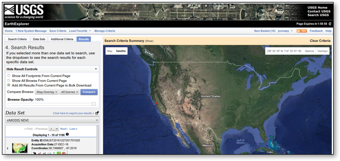
Next, it is possible to select the results from the Search Criteria by selecting “Add All Results from Current Page for Bulk Download” on the “Results” tab and then making the selections. Once that is done, the following steps select the resolution of interest (500 meters) and complete our request for data:
⇒ View Item Basket ⇒ Expand eMODIS NDVI ⇒ Modify Options For All Scenes ⇒
NDVI 500 M ⇒ Proceed To Checkout ⇒ 104.2 GB ⇒ Submit
The USGS Search Results User Interface is shown in Figure 3 below.
Figure 3: USGS Search Results User Interface
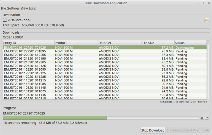
Next, it is possible to download the selected results using the Bulk Download Application (BDA) user interface. BDA is a Java application which is downloaded from USGS and run locally on your desktop or laptop computer. It facilitates the downloading of the large number (in our case, 1166) of fairly large (roughly 100 MB each) files. The Bulk Download Application User Interface is shown in Figure 4 below.
Figure 4: USGS Search Results User Interface
Preprocessing NDVI Data
Once the NDVI data has been downloaded from USGS as described above, the next step is to review the downloaded files and eliminate anomalies. In the example case here, 9 out of 1166 downloaded files were “bad” files - either because they were invalid “zip” files or contained clearly incorrect data.
Once these “bad” files are eliminated, a new PL/R function can be created and executed against the downloaded MODIS data.
The process embodied by this new PL/R function involves loading the area of interest (AoI) administrative boundaries, reprojecting the AoI to same projection as the MOD13A1 raster data, and then looping through the downloaded MOD13A1 NDVI files. For each of the files, the following operations are performed:
- Unzip the File of Interest (FoI), i.e., the current file being processed
- Load NDVI, QA, and Acquisition rasters
- Crop rasters to AoI by trimming the raster matrix to the AoI shape extent
- Mask rasters to AoI by marking cells outside AoI shape boundaries as NA
- Use the QA raster to mark cells with questionable data in NDVI raster as NA
- Use the Acquisition raster to calculate mean date (YYYY.pppp) of NDVI data in the current raster layer
Once these preprocessing operations are performed, it is possible to capture the processed NDVI rasters and dates.
The described preprocessing function is created through the following commands:
loop through all the MODIS files and preprocess
CREATE OR REPLACE FUNCTION process_raw_ndvi
  (mywd text, layername text, name1 text, name2 text)
RETURNS bytea AS $$
  library(raster)
  library(rgdal)
  library(rgeos)

  # initialize
  ingest_dn <- paste(mywd, "/ndvi_raw/", sep = "")
  export_dn <- paste(mywd, "/ndvi_cooked/", sep = "")
  dir.create(export_dn, showWarnings = FALSE)
  ndvi_rast <- raster()
  ndvi_dt <- numeric()
  ndvi_i <- character()

  # retrieve boundaries for requested admin area of interest
  p4str <- "+proj=longlat +datum=WGS84 +no_defs +ellps=WGS84 +towgs84=0,0,0"
  conn <- dbConnect(dbDriver("PostgreSQL"), user="postgres", dbname="gis", host="localhost")
  sql.str <- sprintf("SELECT st_astext(wkb_geometry) AS geom
                                 FROM %s WHERE name_1 = '%s' and name_2 = '%s'",
                               layername, name1, name2)
  aoi <- readWKT(dbGetQuery(conn, sql.str), p4s=p4str)

  # reproject the boundary to the CRS of the MODIS raster
  mp4str <- "+proj=laea +lat_0=45 +lon_0=-100 +x_0=0 +y_0=0 +a=6370997 +b=6370997 +units=m +no_defs"
  aoi <- spTransform(aoi, CRS(mp4str))

  # loop through all of the MODIS raster files
  for (i in dir(path=ingest_dn, pattern="[.]zip$")) {
    # get a list and unzip the files in this archive
    fnoi <- unzip(paste(ingest_dn, i, sep=""), list=TRUE)
    fnparts <- unlist(strsplit(i,'[.]'))
    fnyr <- as.numeric(fnparts[2])
    fndoy <- as.numeric(unlist(strsplit(fnparts[3], "-")))
    unzip(paste(ingest_dn, i, sep=""), exdir = ingest_dn)

    # map the geotiff files to rasterbricks and crop to region of interest
    ndvi <- paste(ingest_dn, fnoi$Name[grep("VI_NDVI.\*tif", fnoi$Name)], sep="")
    r <- brick(ndvi)
    r <- crop(r, extent(aoi))

    qual <- paste(ingest_dn, fnoi$Name[grep("VI_QUAL.\*tif", fnoi$Name)], sep="")
    rq <- brick(qual)
    rq <- crop(rq, extent(aoi))

    acqu <- paste(ingest_dn, fnoi$Name[grep("VI_ACQI.\*tif", fnoi$Name)], sep="")
    ra <- brick(acqu)
    ra <- crop(ra, extent(aoi))

    # mask cells to region of interest
    r <- mask(r, aoi)
    rq <- mask(rq, aoi)
    ra <- mask(ra, aoi)

    # mark cells with questionable data as NA
    r[[1]][(rq[[1]] != 0)] <- NA

    # create raster layer with YYYY.fff for each cell
    if (fndoy[1] fndoy[2]) {
      pfnyr <- fnyr - 1
      len_fnyr1 <- 365 + (pfnyr %% 4 == 0) - (pfnyr %% 100 == 0) + (pfnyr %% 400 == 0)
      len_fnyr2 <- 365 + ( fnyr %% 4 == 0) - ( fnyr %% 100 == 0) + ( fnyr %% 400 == 0)
      sel1 = trunc(ra[[1]] / 100) >= fndoy[1]
      sel2 = trunc(ra[[1]] / 100) < fndoy[1]
      ra[[1]][sel1] <- pfnyr + (trunc(ra[[1]][sel1] / 100) / len_fnyr1)
      ra[[1]][sel2] <- fnyr + (trunc(ra[[1]][sel2] / 100) / len_fnyr2)
    } else {
      len_fnyr <- 365 + (fnyr %% 4 == 0) - (fnyr %% 100 == 0) + (fnyr %% 400 == 0)
      ra[[1]] <- fnyr + (trunc(ra[[1]]/100) / len_fnyr)
    }

    # get mean point in time for represented area
    ra_mean <- mean(ra[[1]][], na.rm = TRUE)
    ndvi_rast <- addLayer(ndvi_rast, r)
    ndvi_dt <- c(ndvi_dt, ra_mean)
    ndvi_i <- c(ndvi_i, i)

    # clean up unzipped files
    file.remove(paste(ingest_dn, fnoi$Name, sep=""))

    # end of preprocessing loop
  }

  ndviout <- paste(export_dn, "ndvi.tif", sep="")
  writeRaster(ndvi_rast, ndviout, overwrite=TRUE)

  return(data.frame(ndvi_i, ndvi_dt))
$$ LANGUAGE 'plr' STRICT;
Note that the PL/R preprocessing function executed above writes the processed
raster layers to a single geotiff file, and returns the data.frame holding the
processed filenames and average corresponding raster layer date to the client in
the form of a binary object. The raster layers could have alternatively been
stored in PostgreSQL tables as PostGIS raster objects.
After the PL/R preprocessing function is created, a new table is created to hold the returned binary object data, and the function is executed with arguments specifying the location of the source raster data and the extraction of San Diego county.
CREATE TABLE robjects(objname text primary key, obj bytea);

INSERT INTO robjects
SELECT 'ndvi_dt', process_raw_ndvi('/usr/local/bda/modis',
                                                                 'counties',
                                                                 'California',
                                                                 'San Diego');
--Time: 8010273.572 ms
Plotting NDVI Data
Plotting the NDVI may now be done with a function similar to the one used earlier to plot Points of Interest. The function below adds a selected, newly processed, NDVI raster layer to the plot. In addition, the administrative boundaries and points of interest are now reprojected to the CRS of the MODIS raster data.
# Note: this is pure R code
plot_poi <- function(rastfile, bricklayer, plotfile, aoilayer, aoiname1, aoiname2, poilayer) {
  library(sp)
  library(raster)
  library(rgeos)
  library(rgdal)
  library(RPostgreSQL)
  Sys.setenv("DISPLAY"=":0.0")

  # CRS of the MODIS raster
  mp4str <- "+proj=laea +lat_0=45 +lon_0=-100 +x_0=0 +y_0=0 +a=6370997 +b=6370997 +units=m +no_defs"

  # required in R, noop in PL/R
  conn <- dbConnect(dbDriver("PostgreSQL"), user="postgres", dbname="gis", host="localhost")

  # plot to file if destination filename given
  if (plotfile != "") png(plotfile, width = 1024, height = 768)

  # retrieve boundaries for requested admin area
  p4str <- "+proj=longlat +datum=WGS84 +no_defs +ellps=WGS84 +towgs84=0,0,0"
  sql.str <- sprintf("SELECT st_astext(wkb_geometry) AS geom
                      FROM %s WHERE name_1 = '%s' and name_2 = '%s'",
                      aoilayer, aoiname1, aoiname2)
  sdc <- readWKT(dbGetQuery(conn, sql.str), p4s=p4str)

  # reproject the boundary to the CRS of the MODIS raster
  sdc <- spTransform(sdc, CRS(mp4str))

  # add county boundaries to plot
  plot(sdc)

  # read and plot requested raster layer
  ndvi <- brick(rastfile)
  ndvi_layer <- ndvi[[bricklayer]]
  plot(ndvi_layer, add = TRUE)

  # retrieve points of interest
  dsn <- "PG:user='postgres' dbname='gis' host='localhost'"
  poi <- readOGR(dsn=dsn, poilayer, stringsAsFactors = FALSE)

  # reproject the poi to the CRS of the MODIS raster
  poi <- spTransform(poi, CRS(mp4str))

  # add poi to plot
  plot(poi, col = "red", pch = 16, add = TRUE)
  if (plotfile != "") dev.off()
}

plot_poi("/usr/local/bda/modis/ndvi_cooked/ndvi.tif", 42, "/tmp/airports2.png",
         "airports", "counties", "California", "San Diego")
The visual result of this command demonstrating the Plotting of NDVI for San Diego County is provided in Figure 5 below.
Figure 5: Visual Results of Plotting NDVI of San Diego County
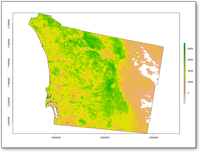
Note the tilted aspect of the reprojected layers. The three airports are still visible as three red dots in a triangular shape in the south-west corner of the county.
Decoding Raster Layer Dates
In order to explore the NDVI data, it is first desirable to convert the stored
data.frame binary object into rows and columns accessible from SQL commands.
The first step in accomplishing that conversion is accomplished by creating a
new helper function that simply returns the desired stored R binary object by
name from the robjects table:
CREATE OR REPLACE FUNCTION get_robj(robjname text) RETURNS bytea AS $$
  SELECT r.obj FROM robjects r WHERE r.objname = robjname
$$ LANGUAGE sql STRICT;
Next, we use the PL/R “modules” feature in order to preload a custom R function into the R environment, so that it might be used by our created PL/R functions:
CREATE TABLE plr_modules (
  modseq int4,
  modsrc text
);

INSERT INTO plr_modules VALUES (0,
$$
  ndvi_d2ts <-function(ndvi_d) {
    fnyr <- as.integer(ndvi_d)
    fnfr <- ndvi_d - fnyr
    daysinyr <- 365 + (fnyr %% 4 == 0) - (fnyr %% 100 == 0) + (fnyr %% 400 == 0)
    fnts <- paste(as.character(fnyr), as.character(round(fnfr \* (daysinyr))))
    as.Date(fnts, "%Y %j")
  }
$$);
The first command above creates a new table called plr_modules. When this
table exists in the specified form, PL/R will use the modseq column to determine
order of execution, and the modsrc column will be evaluated in the R interpreter
which was instantiated for the client session. The value of modsrc in this case
will create a function called ndvi_d2ts() which expects a floating-point
argument that represents a year (the integer part) and a fraction of a year (the
decimal part). The function will create an actual date object in R from the
floating-point value.
The PL/R function ndvi_dates() below will make use ndvi_d2ts(). First, this
function reconstitutes the robj argument back into the originally stored
data.frame. Next, it reformats the second attribute into a real date and
builds a new data.frame that will be returned. PL/R will then convert the R
data.frame into two columns and multiple rows because of the R data type being
returned (data.frame) and the specified PostgreSQL return type (setof record
with two OUT arguments providing the column definition).
Finally when ndvi_dates() is called, the commands use get_robj() to retrieve
the original data.frame from the robjects table and provide it as an argument.
As a result, the original R data.frame is produced in the form of a virtual
SQL table. The timing information is provided to gauge the performance of this
operation, which in this example is reasonably fast.
CREATE OR REPLACE FUNCTION ndvi_dates(robj bytea, OUT lyr_fn text, OUT lyr_date date)
RETURNS setof RECORD AS $$
  return(data.frame(robj$ndvi_i, format(ndvi_d2ts(robj$ndvi_dt))))
$$ LANGUAGE 'plr' STRICT;
SELECT lyr_fn, lyr_date FROM ndvi_dates(get_robj('ndvi_dt')) LIMIT 3;
                           lyr_fn                            |  lyr_date
-------------------------------------------------------------+------------
 US_eMTH_NDVI.2000.056-062.HKM.COMPRES.005.2009221013507.zip | 2000-02-29
 US_eMTH_NDVI.2000.063-069.HKM.COMPRES.005.2009220192553.zip | 2000-03-09
 US_eMTH_NDVI.2000.070-076.HKM.COMPRES.005.2009220130110.zip | 2000-03-11
(3 rows)
Time: 21.937 ms
Conclusion
This series of posts is intended to introduce PostgreSQL users to PL/R, a loadable procedural language that enables a user to write user-defined SQL functions in the R programming language. In particular, this post demonstrated the steps associated with acquiring, preprocessing, and displaying NDVI data from the MODIS TERRA satellite. The coming final post in this series will build on the example introduced in this post in order to demonstrate certain spatial analytic functions.
